Ready-made notebooks

Latest Dynatrace
Reference
1-min read

Dynatrace ready-made notebooks offer preconfigured data visualizations and filters designed for common scenarios like troubleshooting and optimization.

Use them right out of the box
Save a copy and customize your copy

Where to find ready-made notebooks

To list all ready-made notebooks

In Dynatrace, go to Notebooks.
In the Notebooks panel, select Ready-made notebooks.

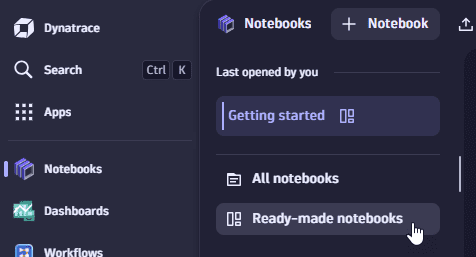Select "Ready-made notebooks"

Alternatively, you can select All notebooks and then change the tab at the top of the table from All to Ready-made.

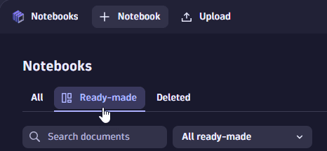Notebooks: Select "Ready-made" tab

Using read-only notebooks

When you open a document (dashboard or notebook) for which you don't have write permission, you can still edit the document during your session. After you're finished, you have two options:

Save your changes to a new document
Discard your changes

Example:

Go to Notebooks, list the ready-made notebooks, and select the Getting started notebook.

It says Ready-made in the upper-left corner, next to the document name.
Select the Line chart section and then select Options.
Change the visualization from Line to Area.

Now you are offered two buttons: Save as new and Discard changes.
Use the updated notebook as needed. You have full edit access for this session.
When you're finished, select what to do with your changes:
- Save as new—saves your changes in a new copy of the edited notebook.
- Discard changes—discards your changes and returns you to the unedited read-only notebook.

Experience Vitals

Explore ready-made notebooks owned by Experience Vitals.

Google Core Web Vitals analysis

Investigate and optimize web performance using Google Core Web Vitals. Analyze LCP, INP, and CLS trends by application to identify performance regressions before they affect users.

The Google Core Web Vitals analysis notebook contains the following sections and tiles:

Application IDs table

The query below will list all of your applications and their associated IDs which can be used further down to filter based on application. To copy the Application ID simply click the cell in the table you want to copy and select 'Copy Value'.
LCP Timeseries Dynatrace Intelligence forecast

The cell below creates a time-series graph of the 75th percentile for LCP across all pages combined over the selected time frame as well as an average value in milliseconds from that timeseries. This view is helpful to understand any significant changes in LCP over the given time frame. If you want to filter to a specific application, uncomment line 3 (ie. remove the ‘//‘) and add your Application ID.
LCP Times per Page and Elements Triggering LCP table

The cell below queries for the 75th percentile of LCP for the slowest 100 pages, groups by the resource URL and identifies the XPath and Tag Name that LCP time.
- CWVs are reported at the page summary event
- All colors for LCP values in the table are aligned with Google's recommendations
If you want to filter to a specific application, uncomment line 3 (ie. remove the ‘//‘) and add your Application ID.
Trending LCP Times per Page line chart

The cell below creates a trending chart that shows LCP times over time by each page URL. This is a useful view to look at longer timeframes and spotlight any baseline changes. If you want to filter to a specific application, uncomment line 3 (ie. remove the ‘//‘) and add your Application ID. Note: the default time for this cell is 24hrs.
INP Timeseries Dynatrace Intelligence forecast

The cell below creates a time-series graph of the 75th percentile for INP across all pages combined over the selected time frame as well as an average value in milliseconds from that timeseries. This view is helpful to understand any significant changes in INP over the given time frame. If you want to filter to a specific application, uncomment line 3 (ie. remove the ‘//‘) and add your Application ID.
INP Duration for Interaction Events at Page Level table

The cell below queries for the 75th percentile of INP for any page and groups by the Element triggering INP, the Interaction Type, and the number of interactions.
- CWVs are reported at the page summary event
- All colors for INP values in the table are aligned with Google's recommendations
If you want to filter to a specific application, uncomment line 3 (ie. remove the ‘//‘) and add your Application ID.
Trending INP Times by Page line chart

The cell below creates a trending chart that shows INP times over time by each page URL. This is a useful view to look at longer timeframes and spotlight any baseline changes. If you want to filter to a specific application, uncomment line 3 (ie. remove the ‘//‘) and add your Application ID. Note: the default time for this cell is 24hrs.
CLS Timeseries Dynatrace Intelligence forecast

The cell below creates a time-series graph of the 75th percentile for CLS across all pages combined over the selected time frame as well as an average value in milliseconds from that timeseries. This view is helpful to understand any significant changes in CLS over the given time frame. If you want to filter to a specific application, uncomment line 3 (ie. remove the ‘//‘) and add your Application ID.
Trending CLS Times by Page line chart

The cell below creates a trending chart that shows CLS times over time by each page URL. This is a useful view to look at longer timeframes and spotlight any baseline changes. If you want to filter to a specific application, uncomment line 3 (ie. remove the ‘//‘) and add your Application ID. Note: the default time for this cell is 24hrs.

Notebooks

Explore ready-made notebooks owned by Notebooks.

Getting started

Interactive introduction to Notebooks. Learn the fundamentals, create data-driven documents, and explore DQL with hands-on examples for analytics and collaboration.

The Getting started notebook contains the following sections and tiles:

Get started with Notebooks

Create powerful, data-driven documents for custom analytics and collaboration. line chart

Explore use case examples on the Dynatrace Playground

Log Analysis Trace Analysis Davis Anomaly Detection Security snippets DQL field extraction examples Davis problem analysis

Users & Sessions

Explore ready-made notebooks owned by Users & Sessions.

Querying of User Events and Session Events

Explore and query user session and user event data. Use this notebook as a reference for DQL patterns to investigate session behavior and user interactions.

The Querying of User Events and Session Events notebook contains the following sections and tiles:

Exploring sessions data table

In many cases, session data may include elements with unclear or inconsistent characteristics. A typical example is a contract number, which may appear in various formats or locations, such as:
- Embedded within a URL
- Stored as a session property
- Assigned as a user tag
Due to this variability, identifying and retrieving relevant sessions can be challenging using standard filters. In such scenarios, the SEARCH command provides a flexible solution. It allows users to query across multiple data fields and formats, making it easier to find sessions based on partial or uncertain information.
Finding sessions with a specific page visited table

Session Events contain basic session data, such as browser name, device, and user tag, and aggregated data such as the number of errors or user interactions during this session.

Data stored in user events must be queried for more precise session finding.

This example displays all unique session IDs of all events that the field url.full contains the phrase "page_of_interest"
What are the top browsers used with my frontend? table

Information about the browser name is stored in User Session events, so it is possible to base on those events. The first step is to filter all sessions that have investigated front-end ID in the dt.rum.application.entities field.

Then the results need to be summarized by browser name and sorted in descending order for clarity.

This type of result is often presented in a pie chart. It can be selected in query options.
Maybe useful later table

Some queries demand joining data from both the user events and session events tables. In this case, user sessions need to be filtered to get only results with a specific user tag. Then, the user event table must be filtered to find those that went through a particular page.

dedup, fields, and limit are helpful to remove duplicates and decide on the fields that should be presented in the table to clarify the results.