Use Grail buckets to partition data

Latest Dynatrace
Overview
6-min read
Published Mar 12, 2026

Use Grail buckets to partition data and help your teams work efficiently, even when they have different data perspectives and requirements. A successful partitioning strategy ensures accurate ingestion, efficient queries, cost-effective retention, and secure access.

This page provides an overview of how to select the best partitioning strategy for your organization. It describes how Grail buckets are used to partition data, and includes use cases to illustrate how to implement this in practice.

Overview

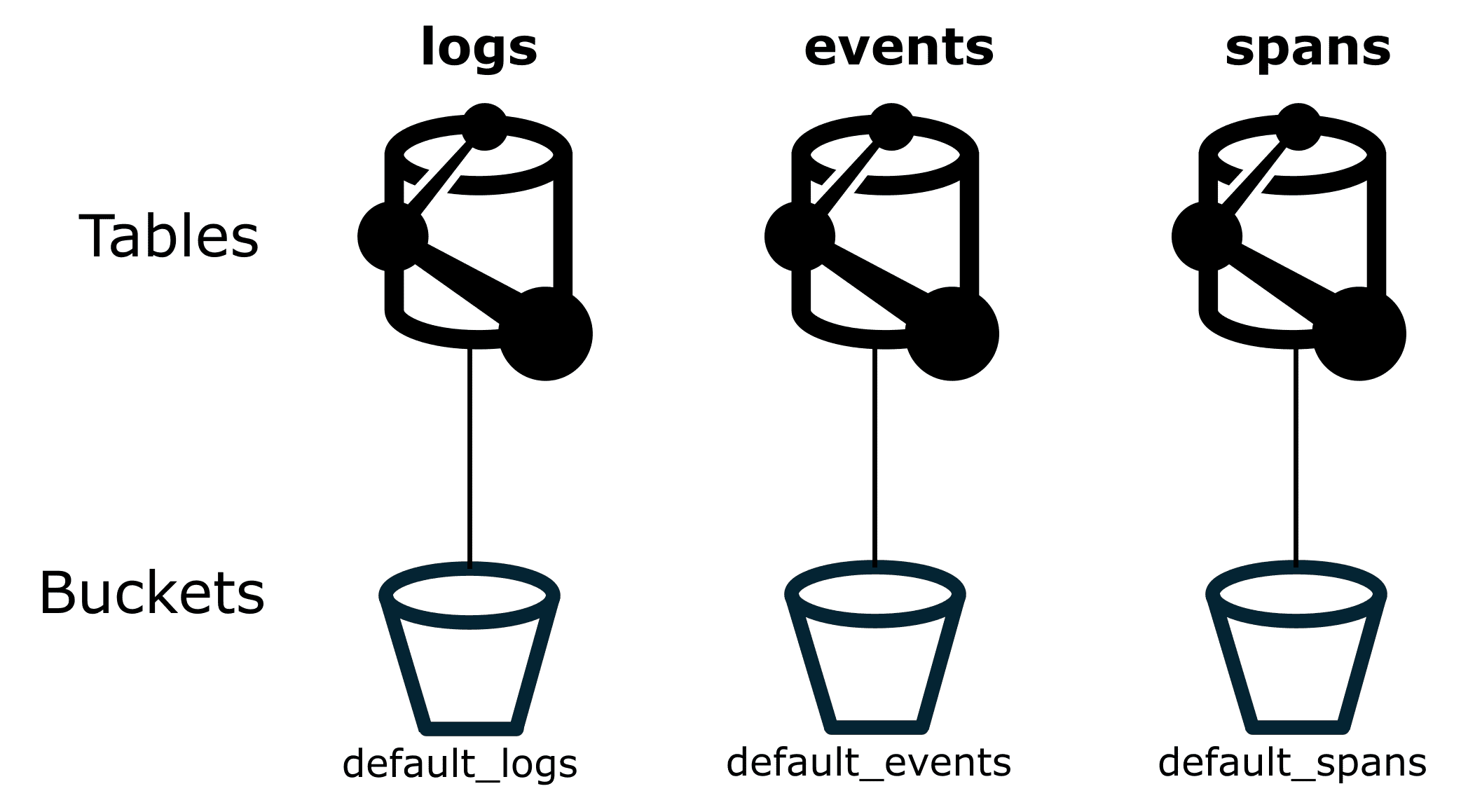
In Dynatrace Grail, table data is physically organized into buckets. Each table is specific to a single record type.

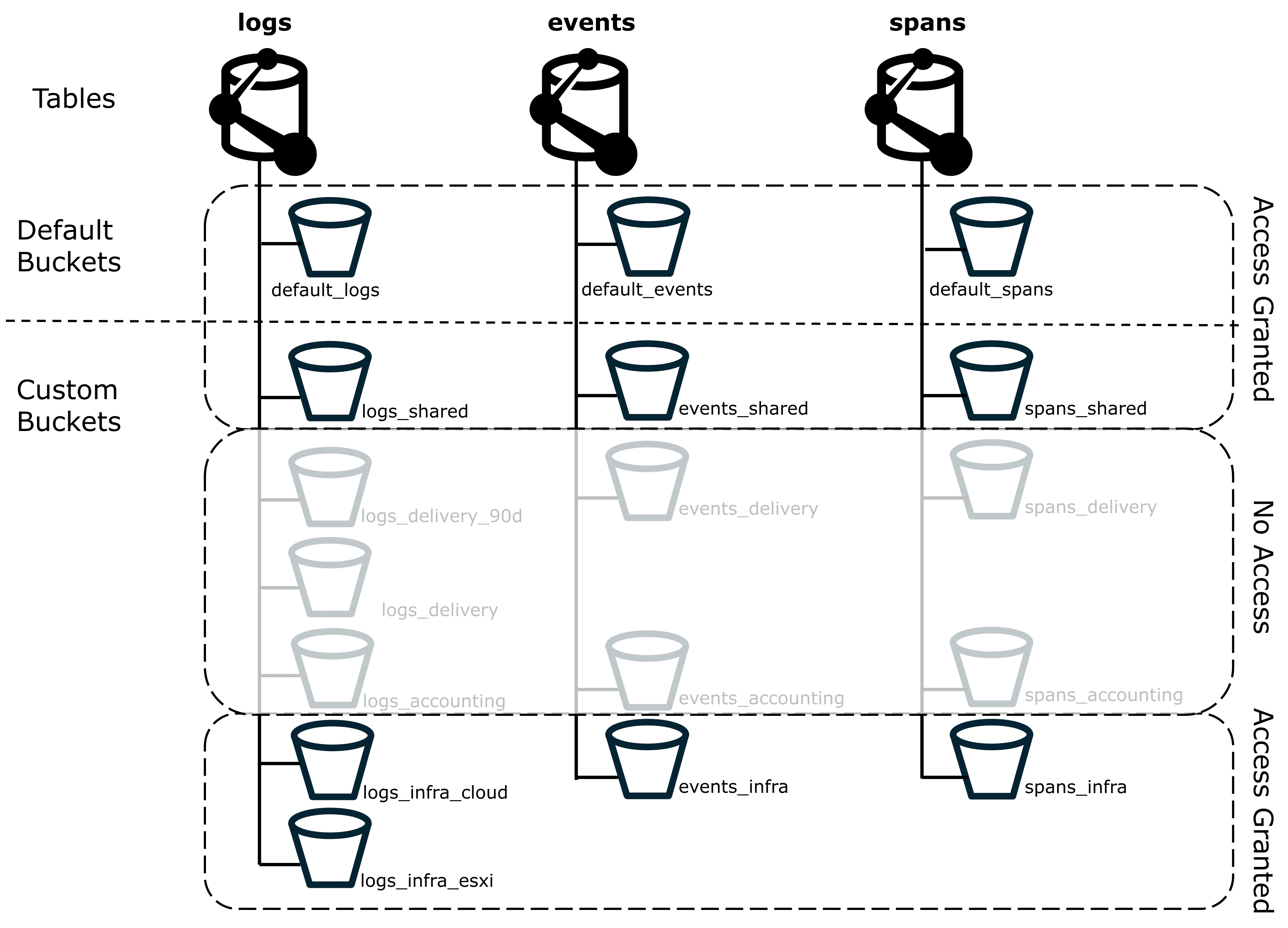
Buckets are the logical storage units where records are stored. Buckets are always associated with a specific record type, such as logs, events, or spans, as shown in the figure below. Dynatrace provides built-in buckets, and you can create custom buckets.

Diagram - Default buckets for different types of table data stored in Grail

By partitioning data into separate buckets, you'll implement the technical foundation that allow advanced data management features:

Retention time management, including custom retention times.
Cost allocation (cross-charging).
Query performance optimization.
Access control.
Data ownership.

Data partitioning strategy ownership

Through experience, we've learned that many of our enterprise customers have central monitoring teams that manage how Dynatrace (and other software) is used across the rest of the teams. Because of this, we recommend that a centralized team also define the overall partitioning strategy. It is vital that this centralized team can evaluate strategy efficiency and adjust as needed.

Many teams produce data, but not all of them own the lifecycle, quality, or retention requirements of that data. In some organizations, the teams that send data into Dynatrace are not the same teams that pay for retention or define retention periods. Make sure these responsibilities are clearly assigned. Clear ownership helps prevent routing issues, avoids unexpected storage growth, and ensures that access privileges stay aligned with actual responsibility.

When designing your partitioning strategy, identify:

Who owns which data?
Who depends on the data?
Who is accountable for retention decisions?

For example, you might want restrict default bucket access to the central monitoring team. By doing this, you can help prevent exposing confidential data to unintended audiences.

Use cases

Read more about how to use buckets to partition data for these use cases:

Partition data according to record type

As a first step, we recommend creating a dedicated set of buckets per record type. You can create custom buckets via either Storage Management or the API, see Manage custom Grail buckets.

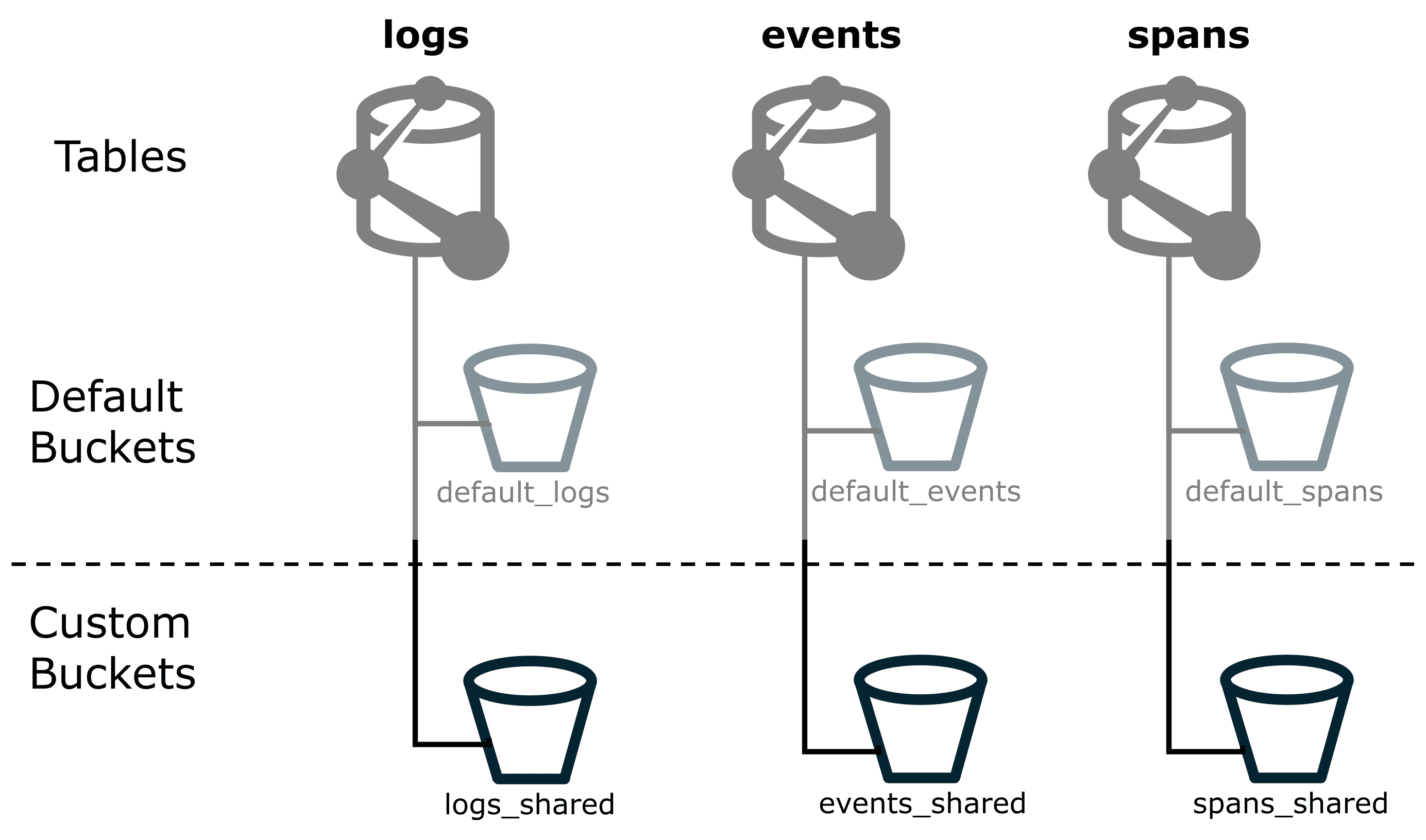
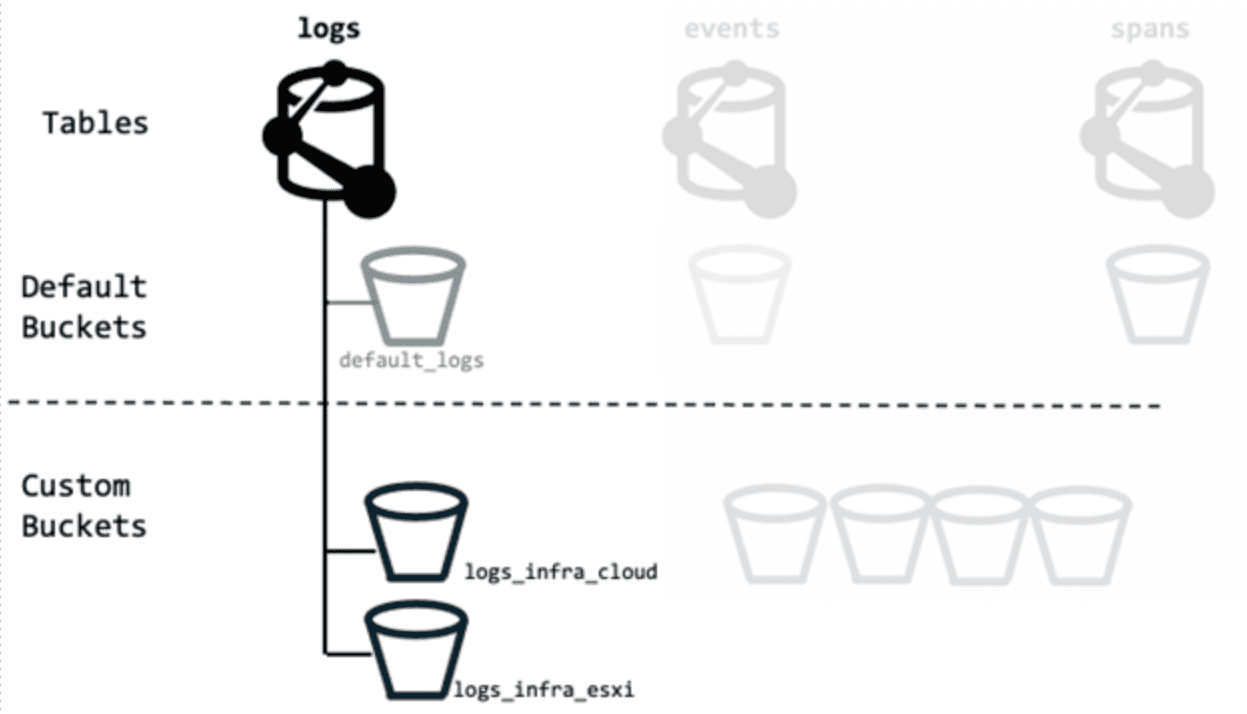
When you create a custom bucket, you can choose a name that best fits your purpose. We recommend:

Have a consistent naming scheme. This, way you always know what kind of data a bucket is supposed to store.
Avoid using default anywhere in the name, because you might confuse the built-in default_logs bucket with a custom logs_default bucket. The figure below shows how you could name custom buckets with _shared as a suffix.

If you haven't specified bucket assignment in the pipeline configuration, Dynatrace will send all ingested data to the default buckets. That means any ingested log lines, for example, will go into default_logs unless the ingest pipeline configuration specifies a different bucket.

While this ensures no data is lost, it doesn't make it easy to tell whether the incoming data is from an already existing monitored component or a service that's just started sending data.

If you configure OpenPipeline so that all known components send their data to your custom buckets, the default buckets should remain empty. If data still appears in a default bucket, it means either that routing was incorrectly configured or that the newly arriving data isn't yet part of the routing setup.

That makes it easy to spot where the data came from, so you can fix the routing, adjust permissions, or drop the data.

Diagram - Partition Grail data with custom shared buckets

Cost Allocation is the process of attributing data storage and query costs to different products or cost centers. You can use buckets to help allocate retention costs, so that the appropriate cost center is billed for their retained telemetry data.

When allocating log retention, Dynatrace can automatically derive cost allocation data from the ingested data, see Allocate your DPS costs. This use case is relevant for all telemetry data.

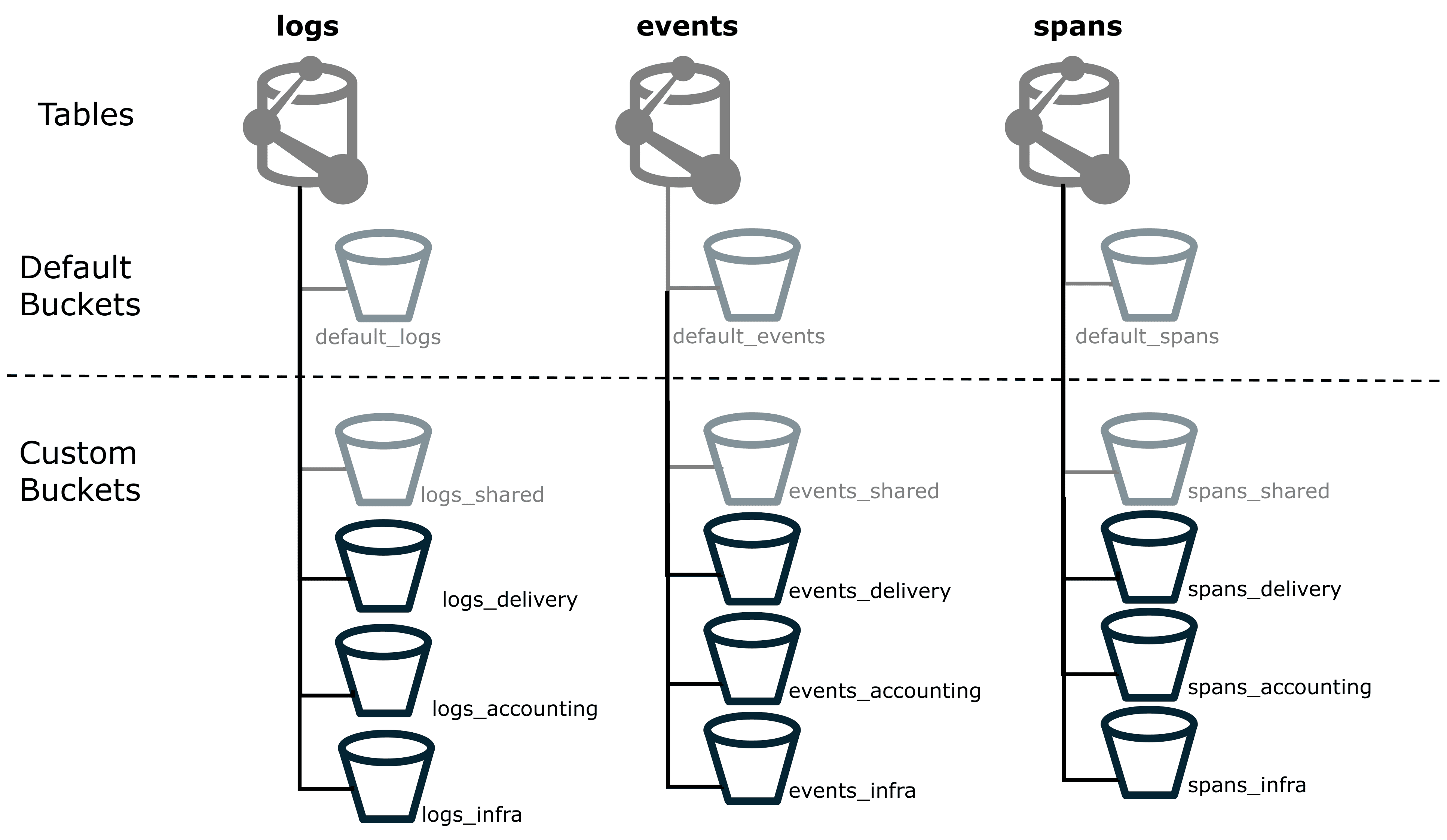
We'll start with the *_shared buckets that we already created, and create additional custom buckets to allocate specific cost centers.

Create a custom bucket for each cost center that you want to allocate costs, see Manage custom Grail buckets. Just like with Cost Allocation via Grail tags, we recommend to name each bucket according to the organizational level to which the costs belong. The figure below shows custom buckets for four different cost centers: shared, delivery, accounting, and infrastructure. We'll do this for logs, events, and spans.
Use OpenPipeline to route all relevant data to the respective cost center bucket, see Processing in OpenPipeline.

Diagram - Partition Grail data into buckets for Cost Allocation

Manage retention time for Grail data

Retention is the length of time that you store data until it is deleted. Different types of data often have different legal, compliance, or business requirements for retention. In Grail, you can configure retention time on a per-bucket basis.

Here's an example of how to use buckets to configure retention time for specific Grail data.

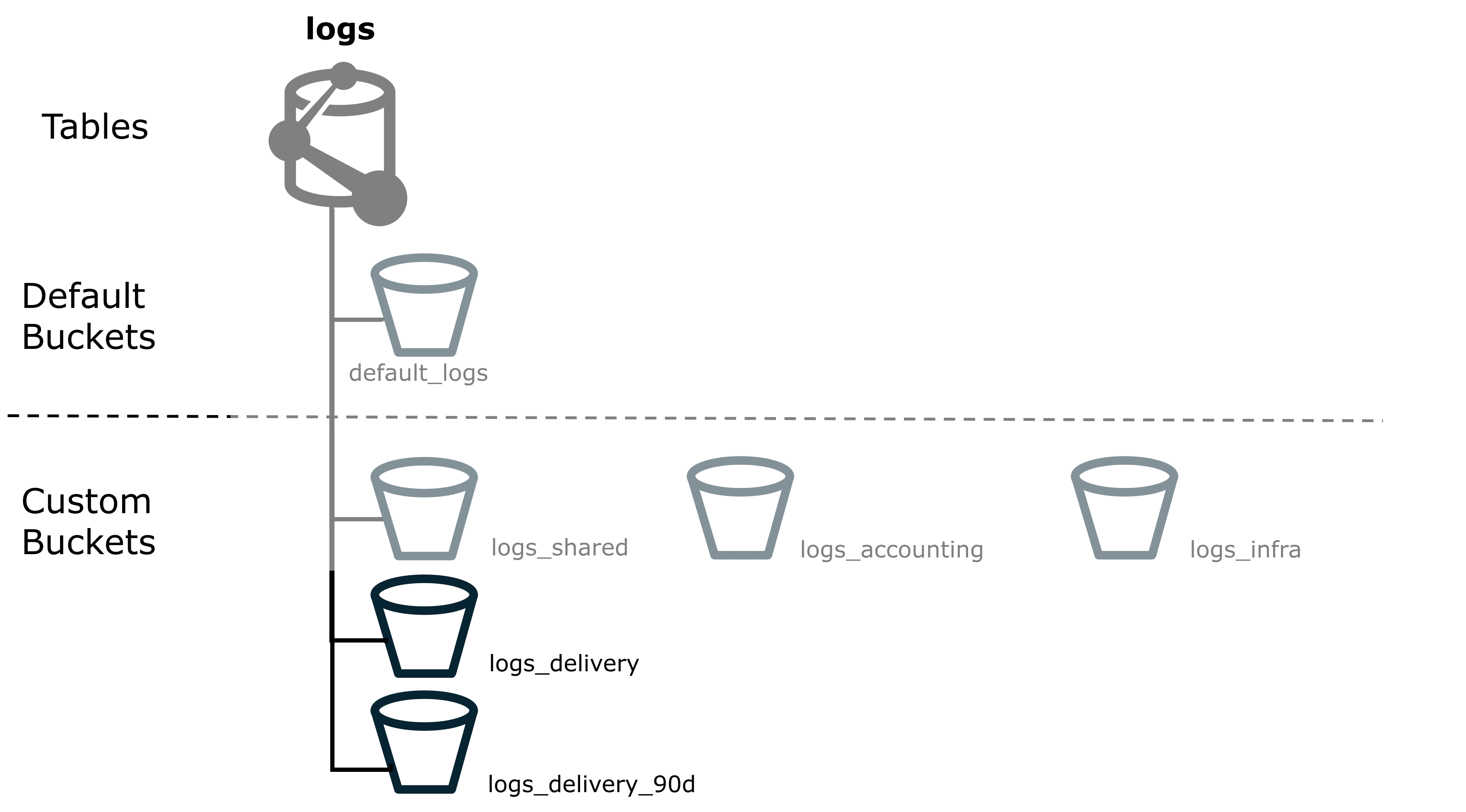
You might have some logs coming from the delivery department, and if these are related to revenue will need to be retained for a total of 90 days. By default, these will all be routed to the logs_shared custom bucket that you created previously.
As these need to be retained for a total of 90 days, create a new bucket named logs_delivery_90d, which clearly indicates the record type, the purpose of the bucket, and the retention time. The figure below shows one logs_delivery custom bucket and one logs_delivery_90d custom bucket.
Set the bucket's retention time to 90 days. The data is saved for 90 days, and then deleted. This guarantees the data is retained, while minimizing total retention costs.

Diagram - Partition data in different Grail buckets to optimize query performance

Optimize DQL query performance

As your data volume grows, efficient querying becomes increasingly essential. The amount of data you ingest per day directly impacts how quickly and cost-effectively you can search and analyze your data.

A successful partitioning strategy does two things:

It effectively distributes data across buckets.
It keeps the number of buckets per query to a minimum.

With the proper strategy in place, a bucket filter is among the most powerful yet simple tools to tune query performance. This how-to guide shows you how to find the buckets that are good candidates for partitioning.

How do you find out which tables in your environment face heavy ingest volume? Query the dt.system.bucket metric to get the currently stored volume and the retention time for all buckets.

Use the query below to get a rough estimate of your average daily ingest.

fetch dt.system.buckets
| filter dt.system.table == 'logs'
| fieldsAdd est_avgDailyIngest = estimated_uncompressed_bytes / retention_days
| fieldsRemove display_name, dt.system.table
| sort avgDailyIngest desc

This query only helps you to estimate your ingest usage. It does not directly relate to your billable ingestion.

Diagram - How a DQL query returns data from Grail buckets

The table below shows an example output from that query.

Name	Retention (days)	Number of records	Uncompressed ingest (bytes)	Daily ingest (GB)
`custom_sen_low_logs_grail_shared`	90	282,678,654,439	797,861,751,782,148	8,865
`default_logs`	35	65,637,645,806	160,968,442,656,818	4,599
`custom_sen_low_logs_platform_service_shared`	90	43,801,831,467	140,559,181,836,772	1,562
`custom_sen_high_kubernetes_istio_network_logs`	365	56,514,903,838	217,887,824,257,262	597
`custom_sen_low_logs_classic_server_feature_shared`	30	6,822,622,009	12,557,657,119,475	419
`custom_sen_low_logs_grail_infrastructure`	90	18,657,828,347	36,640,016,326,373	407

We recommend splitting up buckets that receive more than 2 TB of daily ingest.

Diagram - Partition data in different Grail buckets to optimize query performance

It is up to you to decide which buckets are worth investigating and which criteria make sense for your environment when splitting.

For a broader view over a longer timeframe, feel free to adapt the DQL query. For example, expand your search timeframe to get deeper insights into how the metric has developed over time.
For more advanced analysis and more complex use cases, visit the Dynatrace Community.
We recommend that you avoid relying on any single query or record. If you find a query that has potential for optimization, make sure it has an impact on large sets of data before changing your partitioning strategy.
Fine-tune your DQL queries by following the information at DQL best practices.
Check whether extracting commonly queried log, event, and span content into dedicated metrics makes sense. Querying metrics requires fewer resources and is easier to adapt to than creating buckets.
We recommend periodically reviewing bucket usage and updating your partitioning strategy as query needs evolve.

Control permissions and access to Grail data

Buckets are best used for organizing data by retention time, cost allocation, or query optimization. They are not intended as the primary mechanism for securing or segmenting data access.

While it is technically possible to use buckets to restrict access to specific data, bucket partitioning is not the primary or most flexible method for managing access control in Grail.

Depending on your organization’s structure, access control and Cost Allocation will likely follow similar structural boundaries.

Data access control via IAM

For flexible access control, we recommend to start with record-level permissions, as these will be the best tool for most use cases. In most scenarios, Identity and access management (IAM) provides all the features you need to define who can access which data.

When compared to bucket-based partitioning, permissions offer even greater granularity, finer control, and flexibility. You can easily adapt to changing organizational structures or access requirements without redesigning your data storage strategy. Grail offers record-level and field-level permissions, see Permissions in Grail. For day-to-day access management, we recommend to use Grail record-level permissions.

Bucket strategies for query access control

If your use case requires strict separation of access, start with IAM policies to enforce these boundaries and then use buckets to play a supporting role for very high-level separation (such as isolating highly sensitive data).

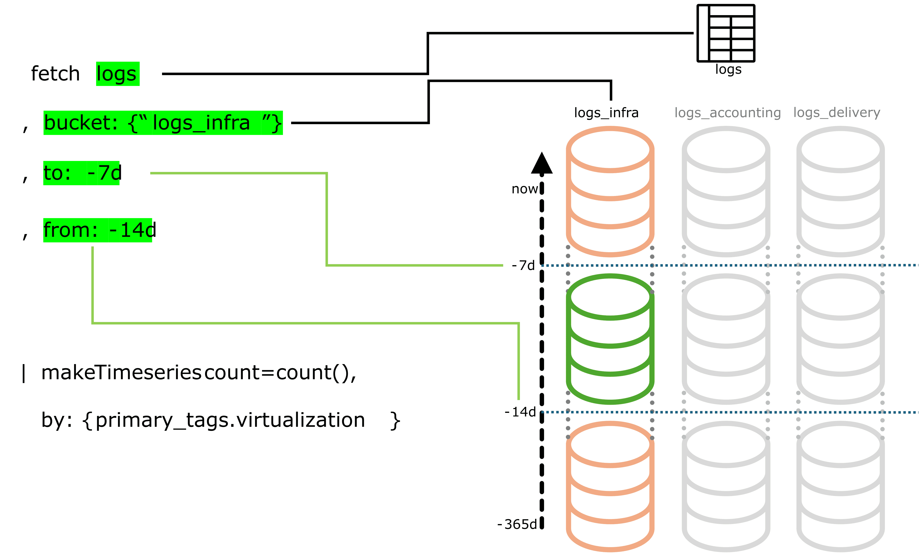
If we want to make sure that users of the infrastructure group don’t have access to delivery or accounting data, we can use the *_delivery and *_accounting custom buckets that we've already created. We can route the relevant sensitive data to these buckets, and use IAM policies to control bucket access. By restricting access at the bucket level, you can ensure that Grail data isn't included in any queries these users execute, including full table scans, as shown in the figure below.

Spans from a single trace can be stored in different buckets. If the user doesn’t have permission for all relevant buckets, the user won't be able to view that trace.

Diagram - Partition data in different Grail buckets for access control

Such access control is only possible with buckets. This is because you can apply a DQL DENY statement to buckets, but not to record-level permissions.

The statement DENY storage:buckets:read WHERE storage:bucket-name="logs_delivery" is valid and denies access to logs in the logs_delivery bucket.
The statement DENY storage:logs:read WHERE storage:dt.security_context="sensitive", however, denies all access to logs, not just those with the sensitive security context.

As a side effect, reducing the number of scanned buckets also improves query performance and reduces query cost. Even if the user didn't have access to see the record, the query would still scan all data in the bucket.

Nevertheless, try to avoid over-complicating your partitioning strategy just to apply specific access controls.

Best practices

Now that you've seen how you can create custom buckets to achieve certain use cases, here are some more things to think about.

Migration from other tools

Migration is a good opportunity to rethink your partitioning strategy. It might be tempting to replicate your previous tool's structure (like Splunk indexes), but keep in mind that Grail buckets have different constraints and capabilities. In Grail, each record can only reside in one bucket, and you can't move data between buckets once it's been ingested.

Partition data with natural query boundaries

You'll always have certain fields that have an extra high number of scanned bytes, when compared to other fields. High-volume fields could include, for example, Kubernetes clusters, cloud account IDs, or applications. These are often natural categories for partitioning data, but not always.

Making one bucket for each Kubernetes cluster (1:1 mapping) sounds simple but it could result in many underutilized buckets, which increases your maintenance workload and the number of scanned buckets per query.
Instead, consider a 1:1 mapping for only the most significant Kubernetes clusters. You can then group the majority of the smaller Kubernetes clusters into a few buckets, or even just one single bucket. This approach is still compatible with strict access control requirements, as it combines bucket and record-level permissions, see Using Grail buckets for access control.

When to use custom buckets

Just because you can add a new custom bucket doesn't mean you should.

For low data volume environments, the default bucket setup is often sufficient.
The most relevant information in deciding when to create a new custom bucket is each bucket's fill rate. For example, a bucket with ingest of 12 TB per day over a one-year period can cause queries and dashboards to time out. While that amount of data in a single bucket can be an intentional decision, it is often a clear indicator of a missing or inappropriate partitioning strategy. You might want to consider routing some data to a different bucket or creating a new custom bucket.
Query performance is dependent on the timeframe and amount of data in the bucket. If you know that you'll only query within narrow timeframes, it's possible ingest ingest well over 15 TB per day into a single bucket without issues. However, longer timeframes in high-volume buckets are more likely to result in slow queries and will yield larger data volumes.
For queries started within apps (such as Dashboards and Notebooks) and workflows, the timeout is 5 minutes. Even if you're fine with slower queries, make sure that the bucket size still allows the query to return data within the timeout limit.
The more frequently data is queried, the more it might be worth storing in a custom bucket. Even if the data volume per query is lower, the higher number of queries will still add up to a higher total cost.
For some use cases there is no alternative to buckets, while for others there is an alternative. Using buckets to achieve each use case (especially if buckets aren't the best solution) has the potential to drastically increase your number of custom buckets, which increases maintenance workload.

Complexity and growth

While there's a lot of flexibility in setting up your bucket strategy, changing an existing setup can be challenging. It's better to start small and to adjust whenever you see proof that it is needed.

Over-engineering the setup early on might lead to rethinking large parts of it later, because expectations didn't align with actual development.
Creating hundreds of buckets manually is tedious and error-prone. We highly recommend using APIs and automation to configure those buckets, in conjunction with a well-defined naming convention.
Short retention times make it easier to adjust your bucket strategy. As data ages out, the legacy structure ages out as well.

Example of successful partitioning

Here's an example model for partitioning that we've seen successfully used by several large customers. Don't take this as a blueprint to copy 1:1, but rather as a starting point for your specific organizational needs.

One Dynatrace customer observes thousands of applications with Dynatrace and has an ingest volume of 250 TB per day. The customer considered creating dedicated buckets for each application, but realized that many would have remained underutilized. Therefore, this wasn't the right choice.

The customer then looked at how these applications are grouped at a higher level. In this case, about 50 different business units were responsible for the applications.

Looking at the numbers, the customer decided to create:

One dedicated bucket per business unit.
Dedicated buckets for applications that still exceeded the recommended daily ingest volume of 2 TB.

This helped them minimize the number of buckets, reducing complexity, while still allowing custom buckets to be created for applications that really needed them.

This example is also relevant when deciding how to partition data with natural query boundaries.

Next steps

Once you've got a partitioning strategy, we recommend familiarizing yourself with OpenPipeline routing and bucket assignments. On their own, bucket definitions are just empty shells. You need to use correct routing to ensure that these buckets are filled with the data that they're intended for.

For more information, see: