Use traces, DQL, and logs to spot patterns

• Latest Dynatrace
• Tutorial
• 14-min read
• Published Nov 20, 2025

Identify abnormal patterns in traces and logs using Distributed Tracing and Dynatrace Query Language (DQL).

Introduction

In this tutorial, you'll learn how to utilize traces, DQL, and logs to:

For your ease of reference, the sections where we use Distributed Tracing are marked with this icon , while the sections where we utilize DQL are marked with . Also, for a detailed explanation of each DQL query, select Explain this DQL query above the DQL query code block.

Target audience

Any user of latest Dynatrace who is eager to learn more about traces, logs, and DQL and understand how to use all these effectively.

Learning outcome

After completing this tutorial, you'll learn how to write and efficiently utilize a variety of DQL queries, which can help you streamline troubleshooting, set up alerts, and automate workflows.

Before you begin

Prerequisites

All you need to complete this tutorial is access to latest Dynatrace in your environment.

Prior knowledge

Identify inefficient database query patterns

Whether a certain SQL statement is executed repeatedly, multiple different SQL statements are called within a trace, or one long-running query is involved—each scenario represents a potential performance issue we aim to detect.

Spot query patterns with Distributed Tracing

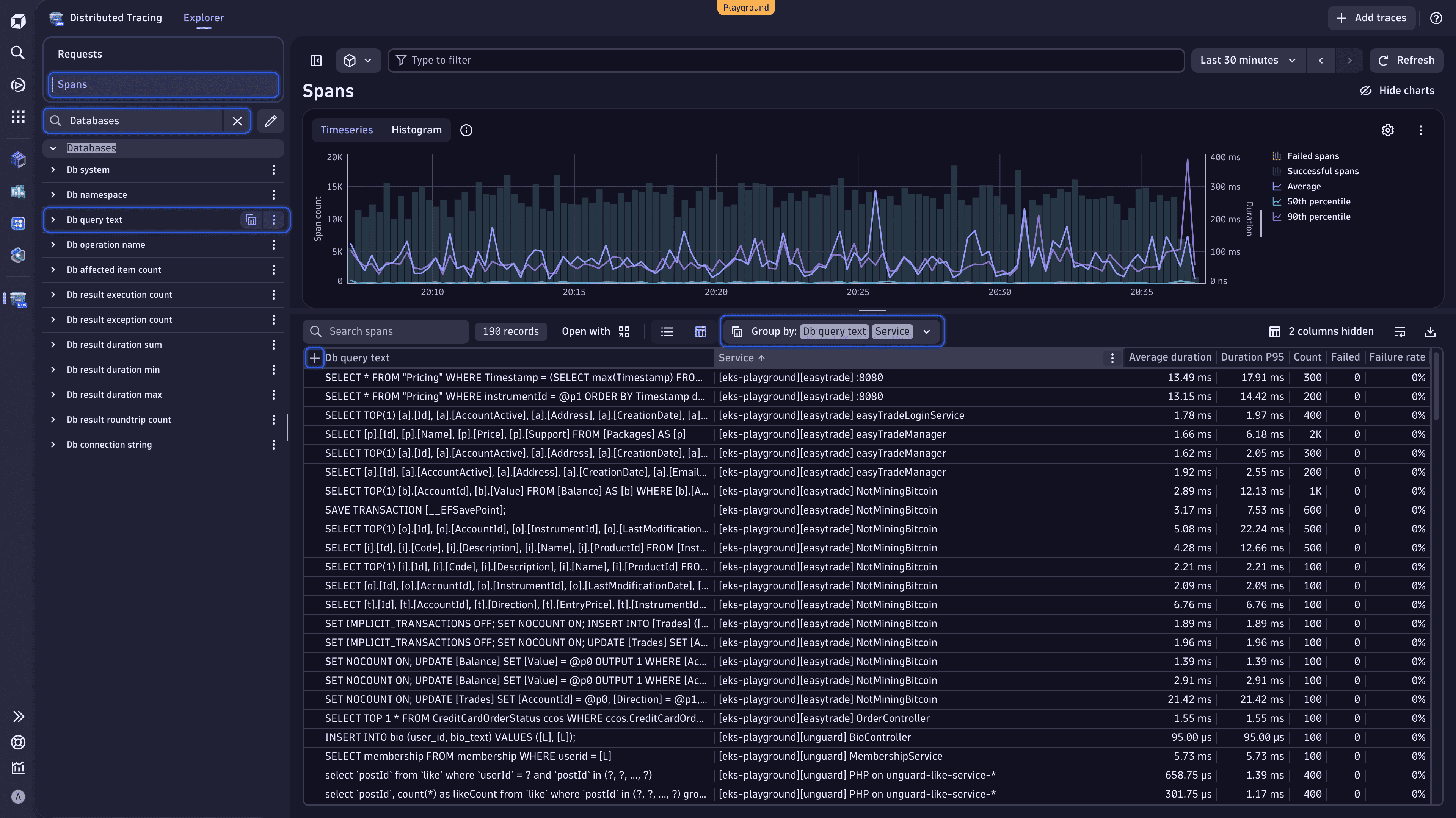
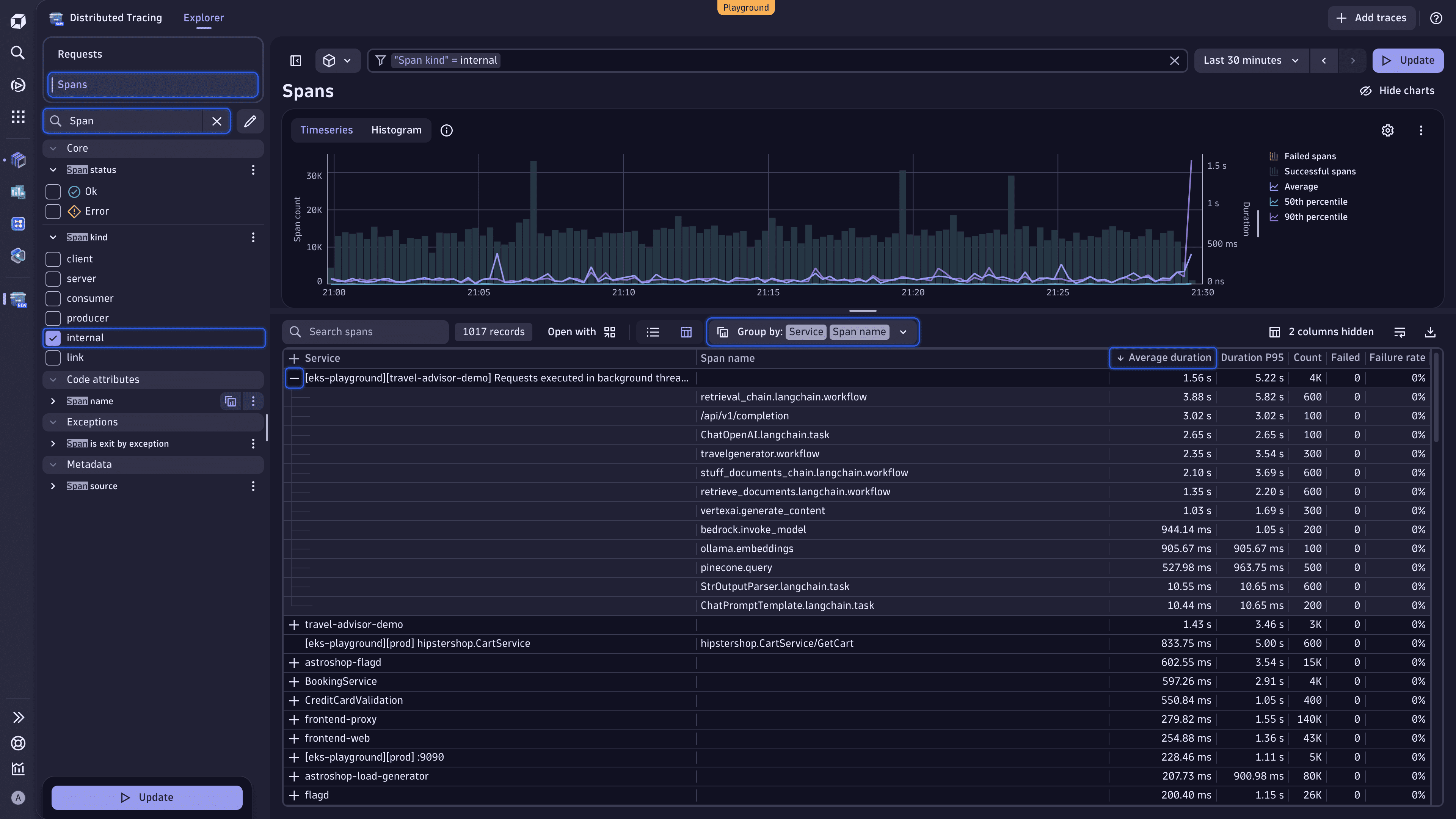
Let's start with Distributed Tracing. Thanks to this app, we can quickly identify inefficient or redundant database usage by leveraging a couple of filters, groupings, and views.

From this view, you can:

Sort data

Select the table column headers to sort the data by different parameters and surface certain database query patterns.

Group data by multiple attributes

Slice your data by multiple attributes to refine your view.

Narrow down data via filters

Apply filters to narrow down the data.

In the Type to filter text field, enter a query. For instance, enter "Db query text" = * to get rid of spans with empty database queries.

Spot unusual patterns with DQL

After utilizing Distributed Tracing, let's learn how to use DQL to reveal atypical patterns in your traces and logs. We recommend using Notebooks to run all the DQL query examples in this tutorial.

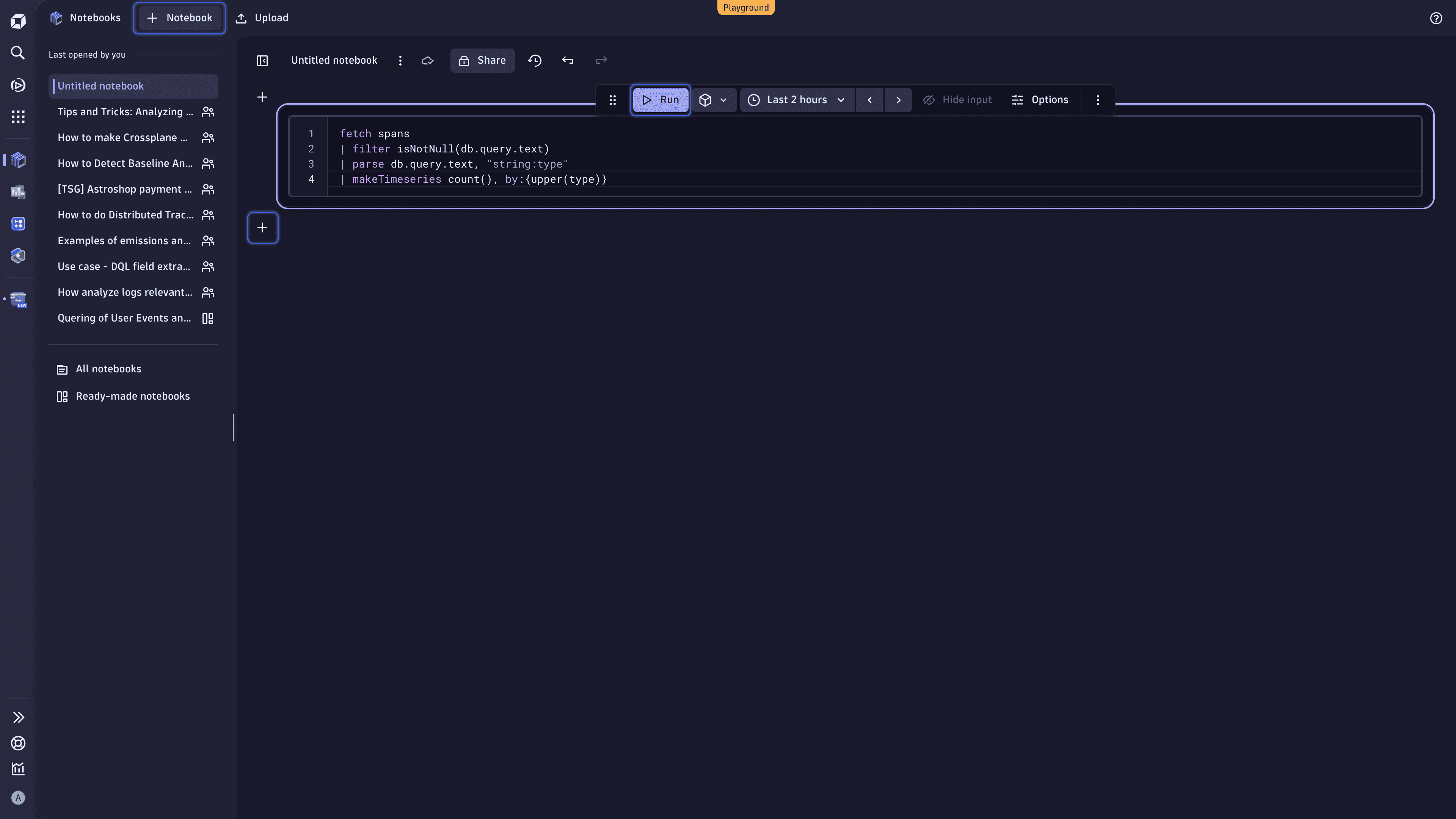
Discover top query types

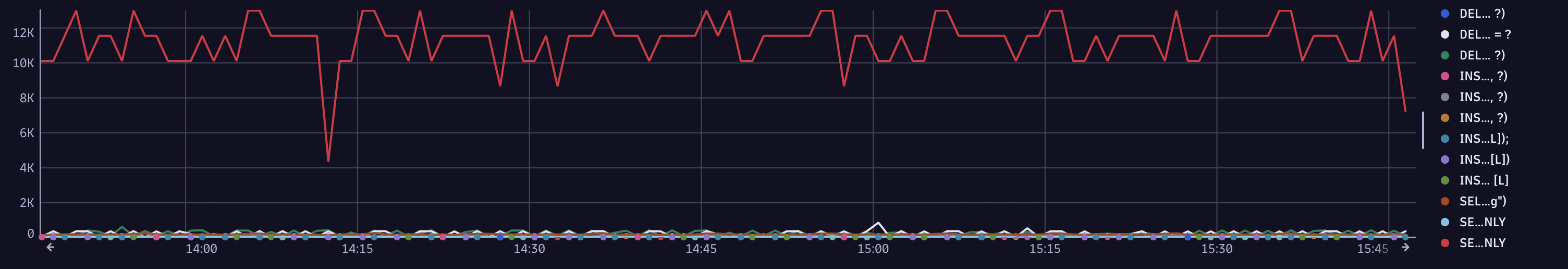
Let's check how often a specific query type (for example, INSERT, SELECT, or UPDATE) shows up in your spans over time. Copy the following query to the notebook query section, and then select Run to execute the DQL query.

fetch spans
| filter isNotNull(db.query.text)
| parse db.query.text, "string:type"
| makeTimeseries count(), by:{upper(type)}

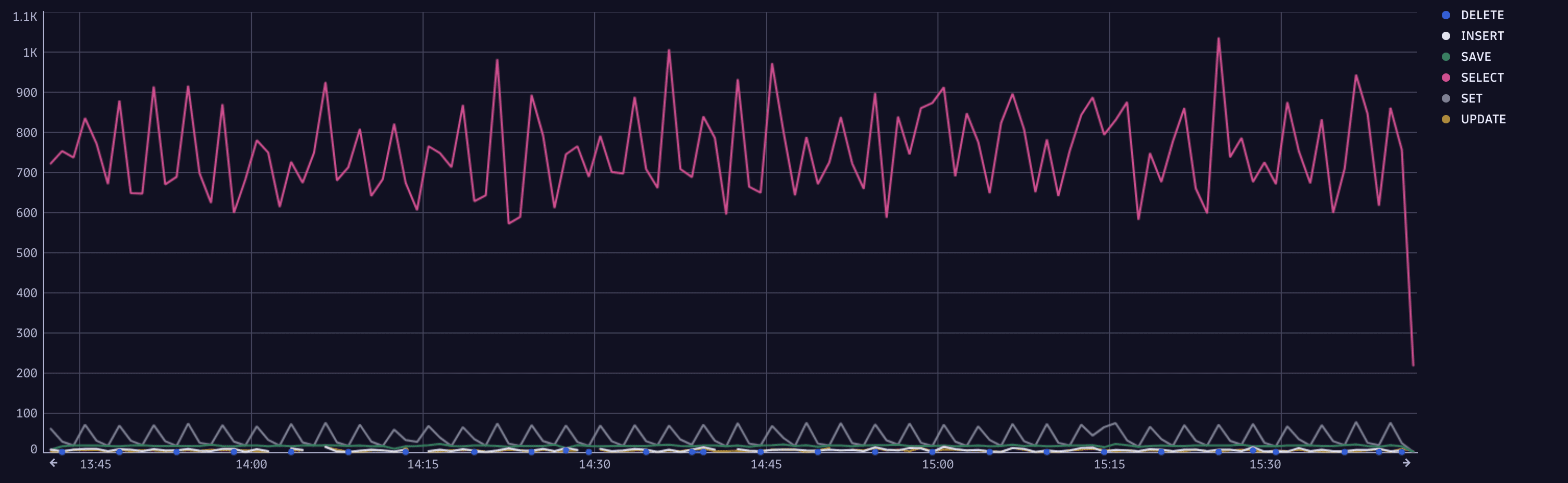
Use this query to understand workload patterns or spot anomalies.

Spot time-consuming queries

Now, let's run the query below to see how long your database queries are taking and locate the slowest queries.

fetch spans
| filter isNotNull(db.query.text)
| makeTimeseries sum(duration), by:{db.query.text}

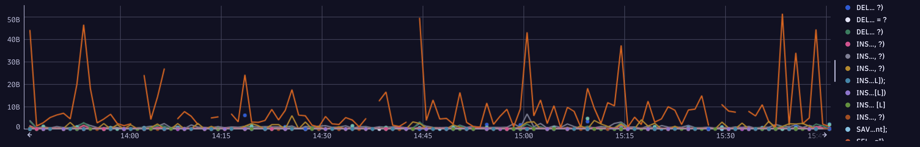
This time series allows us to spot time-consuming database queries and is great for performance tuning. When a query takes too much time, there might be a more efficient query that achieves the same goal.

Reveal high-impact queries

With this query, we can check how many rows of data are affected—for example, SELECTed, INSERTed, or DELETEd—by each database query.

fetch spans
| filter isNotNull(db.query.text)
| makeTimeseries sum(db.affected_item_count), by:{db.query.text}

This time series shows how many rows of data are affected by each query. If a particular query affects more data rows than others, such a query would be a great candidate for optimization.

Spot exception patterns

In this section, let's use DQL to reveal certain exception patterns. We'll determine which exception types are most common and locate services with the most exceptions.

Count exceptions per exception type

We focus on the number of exceptions that are coming in and learn how frequently each type of exception occurs.

fetch spans
| filter iAny(span.events[][span_event.name] == "exception")
| expand span.events
| fieldsFlatten span.events, fields: {exception.type}
| makeTimeseries count(), by: {exception.type}, time:start_time

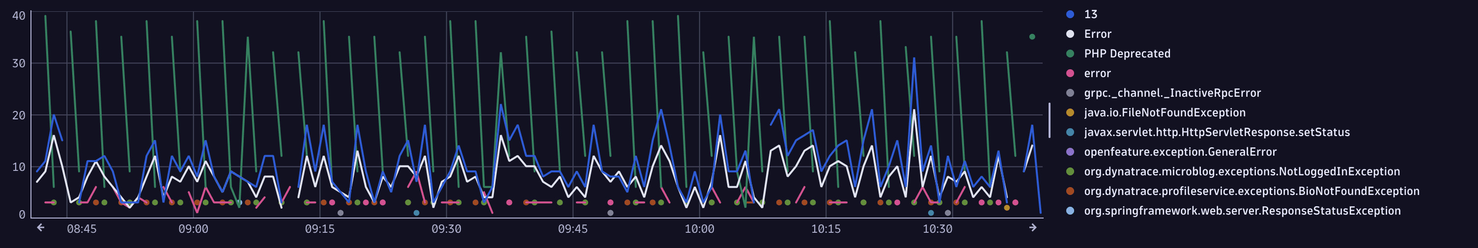
Checking the number of exceptions per exception type can be useful for error monitoring and debugging. With this query, you can:

Spot services with most exceptions

With the next query, we get the list of services with the largest number of exceptions.

fetch spans
| filter iAny(span.events[][span_event.name] == "exception")
| expand span.events
| fieldsFlatten span.events, fields: {exception.type, exception.message}
| summarize count(), by: {service.name, exception.message}

Spotting services with the highest number of exceptions can help you triage and prioritize your team's troubleshooting efforts. Moreover, knowing which exception messages are most common can help you detect recurring bugs or misconfigurations.

Detect hotspot internal methods

When it comes to code optimization, you might first want to see what your hotspots methods are. In this case, we can analyze all spans that represent internal method calls and then group them by service and span name.

Find long-running spans with Distributed Tracing

Here is how we achieve that in Distributed Tracing.

You can instantly see which spans are consuming the most time.

Identify top 10 slowest internal spans

Leveraging the next query, you get the list of slowest internal span nodes by average duration.

fetch spans
| filter matchesValue(`span.kind`, "internal")
| summarize {durationSum = sum(duration), callCount = count(), avgDuration = avg(duration)}, by: {service.name, span.name}
| sort avgDuration desc
| limit 10

Identifying a function in your code that consumes a significant amount of execution time or resources helps detect bottlenecks, understand runtime behavior, and streamline optimization efforts (such as reducing CPU usage, memory consumption, or response time).

Identify log patterns: services with most logs

Now, let's unveil services that produce the largest number of logs. The query below offers us a simple way of identifying our top log producers within the context of a trace.

fetch logs
| filter isNotNull(trace_id)
| summarize count = count(), by: {service.name}
| sort count desc
| limit 20

Such a DQL query comes in handy when you need to understand which services produce the largest number of logs. Knowing that, you can identify log-heavy services, which might be over-logging, and optimize log ingestion costs.

Join logs and traces: count logs per service endpoint

Finally, let's find out how many logs are created per service endpoint.

By default, logs don't contain endpoint information. However, by enriching logs with the trace ID, we can join logs and traces based on their common field.

fetch spans
| join [
    fetch logs
    | fieldsAdd trace.id = toUid(trace_id)
    | summarize logCount = count(), by: {trace.id}
], on: {trace.id}
| filter isNotNull(http.url)
| summarize {requestCount = count(), logCount = sum(right.logCount)}, by: {http.url}
| fieldsAdd logPerRequest = logCount / requestCount
| sort logPerRequest desc

Running this query, we obtain a list sorted by endpoint that summarizes the number of requests and logs received for each endpoint, while we also calculate the ratio of logs per request. This is useful in identifying our heavy-hitting endpoints that might be producing excessive logs.

Call to action

We hope this tutorial has given you some additional tips and tricks on how to become more efficient in analyzing traces and logs and spotting abnormalities in your environment. You can apply similar techniques to exceptions, hosts, processes, remote procedure calls, and more.

You learned how to use Distributed Tracing to detect database query patterns. Furthermore, you grasped numerous examples on how to utilize DQL to find services with the most exceptions, identify hotspot methods, and even join logs and traces to calculate the number of logs created per service endpoint.

If you believe that you need to have certain information at hand, add the DQL query result to the dashboard. You might also consider creating a metric that you can extract from the logs as they come into Dynatrace.

Next steps