Seasonal baseline

A seasonal baseline represents a dynamic approach to baselining where the systems have distinct seasonality patterns. An example of a seasonal pattern is a metric that rises during business hours and lies low outside of them. For such a case, it is difficult to set up an alerting configuration based on a static or auto-adaptive threshold. If you set a fixed threshold based on business hours' behavior, you'll miss an anomaly outside of business hours. Davis® AI learns the seasonal behavior of your metrics and automatically creates a confidence band for it.

When the configuration of a metric event includes multiple entities, each entity receives its own seasonal baseline, and each baseline is evaluated independently. For example, if the scope of an event includes five services, Dynatrace calculates and evaluates five independent baselines.

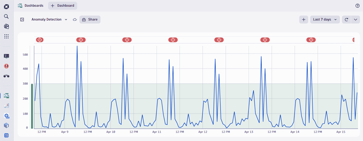
Baseline example

Let's check an example where a seasonal baseline has an advantage over a non-seasonal threshold. The chart below shows the measurement of the user actions of an application. As you can see, there are daily peaks at about 8 AM. When evaluated by an auto-adaptive threshold, those peaks result in false positives (red marks above the chart).

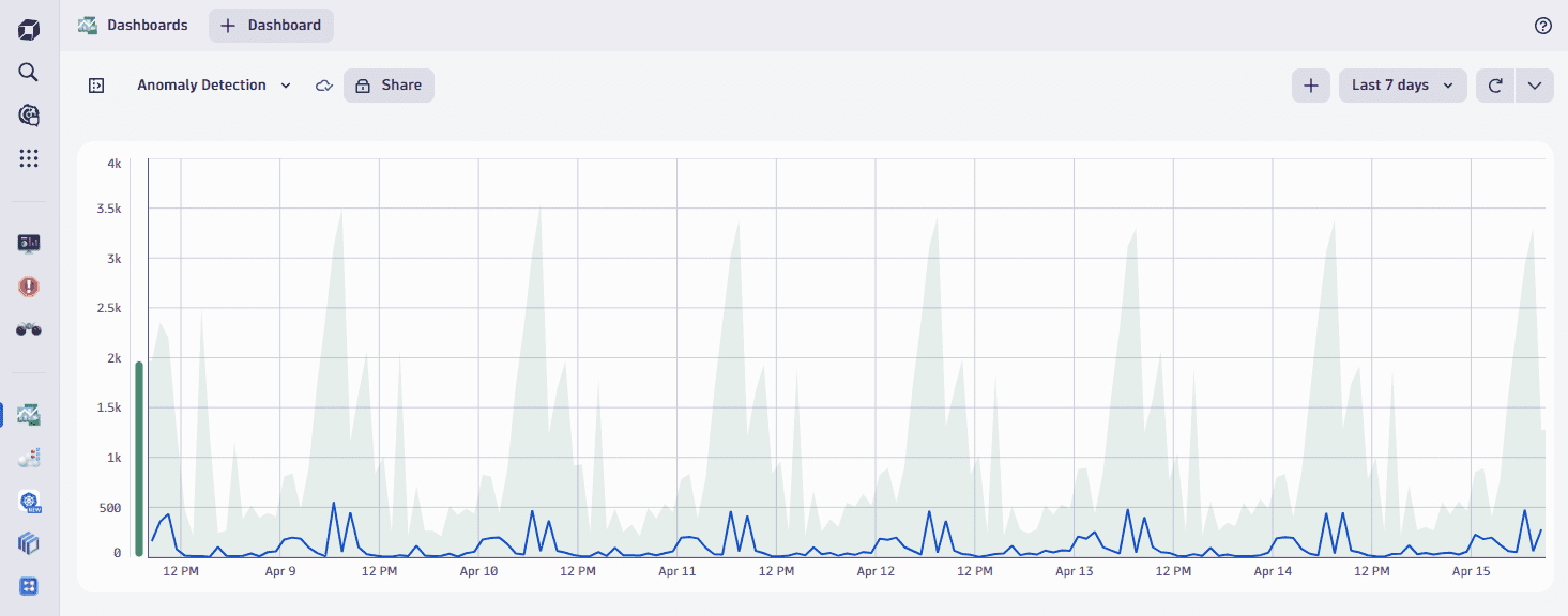
Davis AI automatically checks if the seasonal model conditions fit and creates a confidence band based on the seasonal pattern. As you can see on the chart below, the model recognizes seasonality and doesn't generate false alarms on the peaks. However, it will still trigger an alert should a spike occur at a different time.

Parameters of the baseline model

The seasonal baseline model uses the metric values for each minute during the last 14 days as the reference for the baseline calculation. The model learns the usual behavior of the metric and aims to detect regularly repeating patterns. It uses probabilistic prediction to compute the confidence band, which covers the expected range of a future point.

You can adapt the width of the confidence band via the tolerance parameter. A higher tolerance means a broader confidence band, leading to fewer triggered events. The allowed range for the tolerance is from 0.1 to 10, with 4 as the default value.

As the name suggests, the seasonal model is beneficial for data with seasonal patterns (for example, daily peaks). As it consumes significant resources and needs more time to learn the behavior, there are some validation checks to ensure optimal performance. The validation evaluates each tuple (unique combinations of metric—dimension—dimension value). If there's no pass, a simple model is used instead, with the respective message appearing in the preview.

The simple model calculates the confidence band based on the robust estimation of the distribution of the input data and its calculated interval stays constant over time. For the simple model, the tolerance parameter controls the width of the confidence band in the same manner as for the seasonal model.

If metric boundaries (minimum or maximum value of the metric) are set in the metric metadata they are automatically considered in the model. If no metric boundaries are set and the input data contains only positive values, the model automatically sets a minimum boundary value of 0. If a minimum or maximum value is found, the confidence band does not exceed this value.

The model (be it seasonal or simple) is updated daily.

Another important parameter for seasonal baselines is the sliding window that is used to compare current measurements against the confidence band. It defines how often the confidence band must be violated within a sliding window of time to raise an event (violations don't have to be successive). This approach helps to reduce the number of false positives when alerting. You can set the sliding window to a maximum of 60 minutes.

Training of the baseline model

The seasonal baseline model uses the metric values for each minute during the last 14 days for training and is trained per tuple (unique combinations of metric—dimension—dimension value). The training happens on daily basis.

The image below provides an overview of the training process.

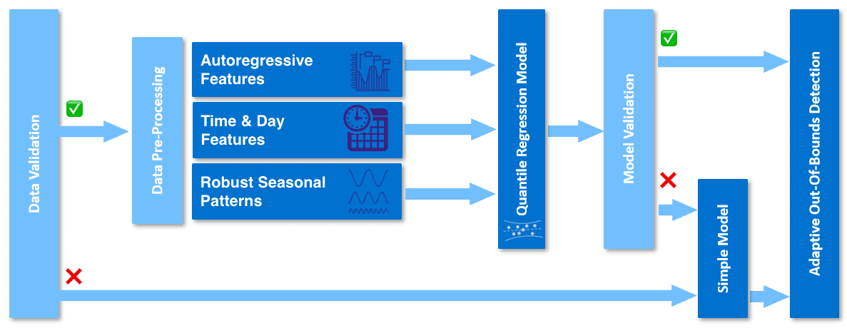
The first step, data validation, ensures that it is reasonable to train a seasonal model on the metric data. Here are some reasons to switch to a simple model:

If this validation fails, the simple model is used instead. If the validation is successful, the next step is the pre-processing of the input data. In this step the data is prepared for training the quantile regression model which learns the seasonal behavior from three main characteristics (features) of data:

These features are used to train the Quantile regression model, a probabilistic regression model, that is robust against outliers due to estimating quantiles.

The next step is the Model validation, which verifies the reliability of the forecasted quantiles on a subset of data. If this validation fails, the simple model is used instead.

After the training is finished, Dynatrace uses the seasonal model to detect anomalies. Each minute the model produces a one-step-ahead forecast of the confidence band for the next minute. Once the actual data point arrives, the predicted confidence interval is compared with the actual value to check whether the value is within the predicted boundaries.