Dynatrace Intelligence predictive AI analysis
- Latest Dynatrace
- Explanation
- 14-min read
The forecast analysis predicts future values of any time series of numeric values. The forecast analyzer is not limited to stored metric data—you can bring your own data, use a metric query, or run a data query that results in a time series of numeric values.
The analysis is agnostic to the distribution of the input data. The forecast is calculated without any assumption about specific data distribution and works for both symmetric and non-symmetric distributions.
You can trigger a forecast analysis from your notebook.
Analyzer input
| Parameter | Description |
|---|---|
Time series | Input time series serving as the base for the prediction analysis. It must include at least 14 data points. If fewer than 14 data points are available, the forecast fails. |
Number of simulated paths | The number of paths (nPath) simulated by the sampling forecaster. The more paths that are simulated, the more accurate the forecast and the longer it takes to calculate. The default value is |
Forecast horizon | The number of data points to be predicted. The more data points that are predicted, the less accurate the forecast is. The default value is |
Coverage probability | The coverage probability targeted by the forecaster, which translates to the following quantiles:
where For example, if the coverage probability is The default value is |
Forecast offset | The number of most recent data points that are ignored by the forecaster. The offset helps you to exclude incomplete data points from the forecast, since because incomplete data has a negative impact on the forecast. The default value is |
Analysis methodology
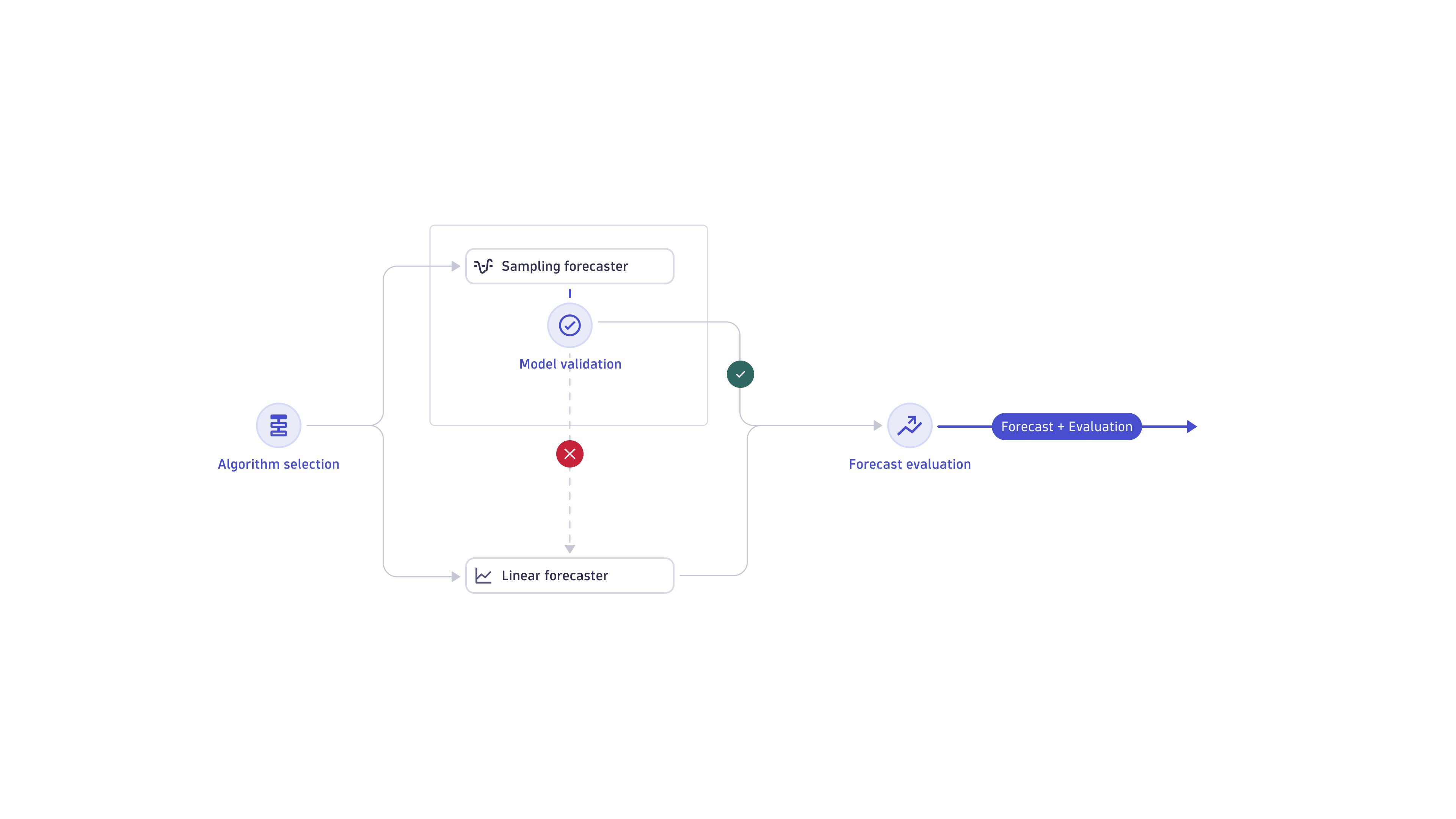
When you trigger a forecast analysis, the time series is sent to an appropriate forecaster that produces the forecast. Then the forecast quality is evaluated, and the forecast and evaluation are returned as analysis results.
Algorithm selection
The analysis uses one of the two forecasters:
The sampling forecaster is used if the variance of the linear history timeframe is larger than the maximum value of the 0.1 and 0.001 × input time series variance pair. The linear history timeframe is the X most recent data points, with X being in the range from 14 to 20.
In any other case (including the case when training of the sampling forecaster fails), the linear extrapolation forecaster is used.
Sampling forecaster
The sampling forecaster provides multi-step forecasts based on seasonal patterns. Its architecture is shown in the image below.
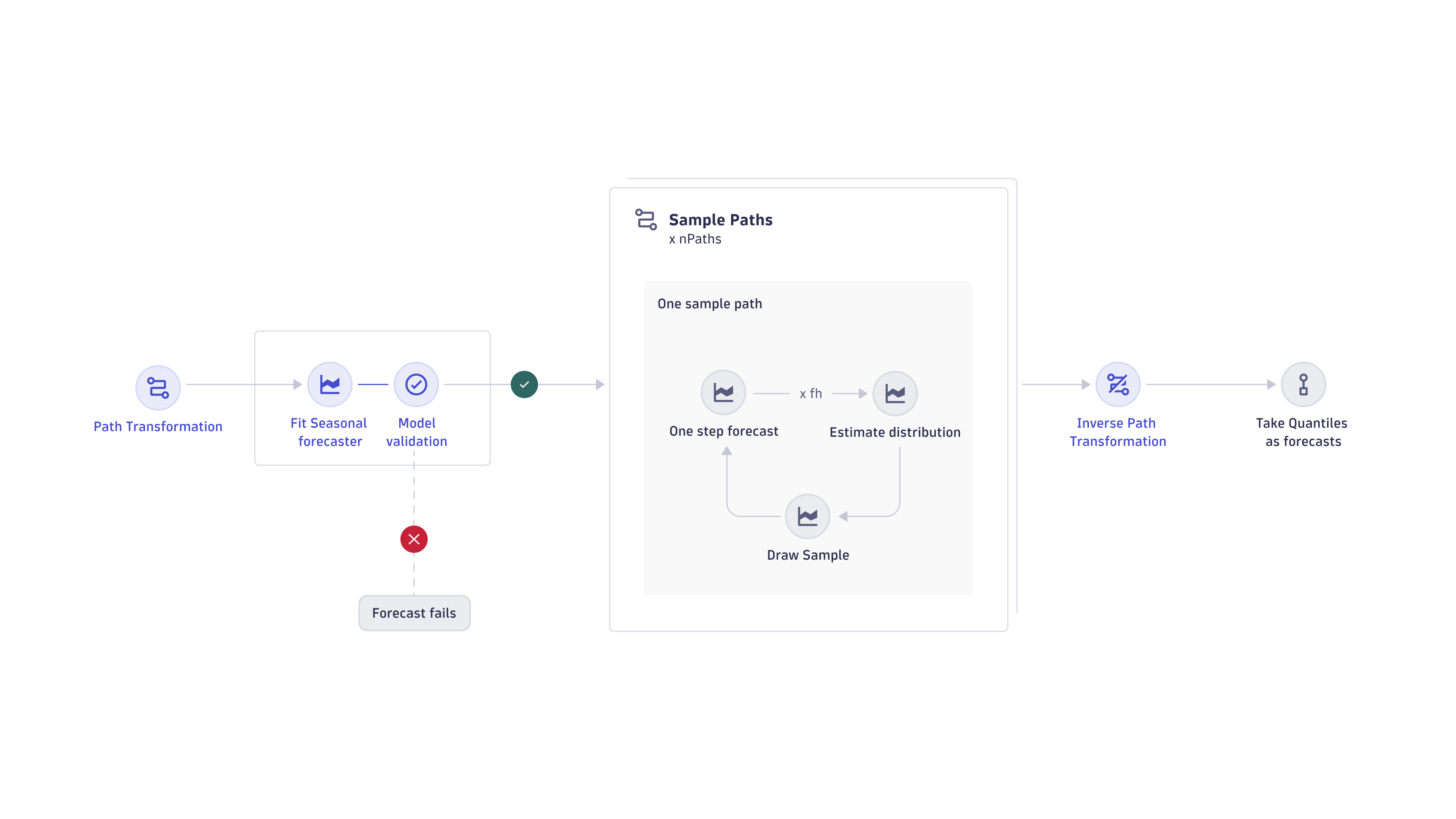
First, the path transformer is applied to the input time series, and then the forecaster is trained on it. If the resulting model is invalid, the linear extrapolation forecaster is used instead. If the model is valid, sampling paths are created by the seasonal forecaster. Those paths are then inverse transformed before applying the quantiles on each time step.
Seasonal patterns
The forecaster always looks for various seasonal patterns in the input time series. The input time series must contain enough data to detect seasonality reliably.
| Seasonal pattern | Required time series duration |
|---|---|
1 hour | 2+ hours |
1 day (24 hours) | 7+ days |
1 week (7 days) | 14+ days |
Day of week | 7+ days |
Time of day | 2+ days |
Minute of hour | 2+ hours |
Apart from those natural patterns, the forecaster looks for any repetitive patterns in the time series by breaking them based on a certain time window.
Forecast step-by-step
-
The seasonal forecaster estimates quartiles of the time series distribution at the time stamp of the next data point.
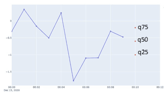 Multi-step prediction algorithm - step 1
 -
The distribution for the value at the next time step is estimated from the quartiles. The bell curve in the image is for illustrative purposes and doesn't represent the distribution used in the sampling forecaster.
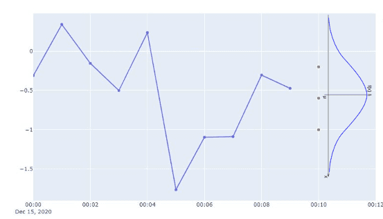 Multi-step prediction algorithm - step 2
 -
The value for the next time step is sampled from the distribution obtained in step 2.
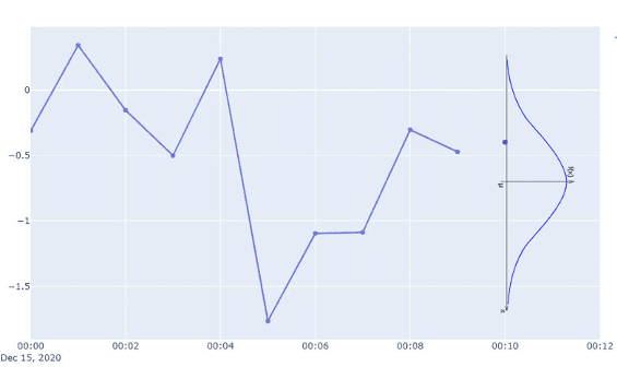 Multi-step prediction algorithm - step 3
 -
The value obtained in step 3 is now considered a part of the time series, and the forecaster repeats steps 1 to 4 until it reaches the forecast horizon.
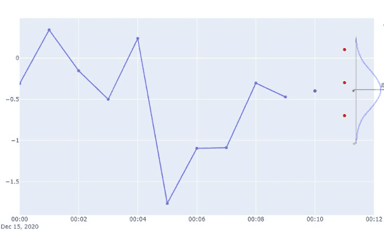 Multi-step prediction algorithm - step 4
 -
The predicted data points form a single sampling path (shown in red in the image below).
 Multi-step prediction algorithm - step 5
 -
The forecaster repeats this process N times, creating multiple sampling paths.
 Multi-step prediction algorithm - step 6
 -
The forecaster takes the sought-after quantile at each time step, forming the prediction interval (shown in light purple in the image below).
 Multi-step prediction algorithm - step 7
Linear extrapolation forecaster
The linear extrapolation forecaster is an algorithm that uses simple linear regression to find the best-fitting line through a number of data points and extend this line into the future. The number of data points used to train the forecaster is determined as follows

where n is the length of the input time series.
To train the linear extrapolation forecaster, nHistory must contain at least 14 non-null data points.
For the sake of simplicity, we calculate the confidence interval under the assumption that the residuals are normally distributed as follows:

where tcrit is the 95th percentile of the Student's t-distribution. The standard error is

where X̅ is the mean value of x, the sums taken over the training data, and s is the sample standard error of the last nHistory points of the input time series.

Forecast quality assessment
After the predictions are generated, we assess their quality to spot potential numerical problems. To assess the forecast quality, the analyzer compares the standard deviation of the prediction to the standard deviation of the input time series (SDinput).
The standard deviation of the predictions (SDprediction) is calculated as the maximum standard deviation of the lower and upper bounds of the prediction interval as well as the standard deviation of the point prediction.
To account for acceptable trends in the predictions, the analyzer uses a scaling factor (SCF). When the length of the prediction data (Nprediction) is large compared to the input time series (Ninput), we allow a larger standard deviation of the prediction than for a small prediction.
Additional input into the scale factor is the Standard deviation factor (SDfactor), with a default value of 100. The scale factor is calculated as follows:

The forecast is evaluated by the following condition:

If the condition is satisfied, the forecast is assessed as valid. Otherwise, the forecast is invalid.
Write DQL queries for forecasting
When using the forecast analysis in one of your notebooks, you can write any DQL query that returns time series data in the time series record format.
- If the data does not comply with one of the above formats, the forecast analysis fails.
- Every numerical value in a data array must have at least one decimal point (for example,
1.0).
Example queries
The example DQL queries below yield valid responses.
-
The
timeseriesDQL command always returns a response in the time series record format. -
You can also write queries using the
fetchcommand together with thesummarizecommand. Those queries will return data in the single value format. All records must have the same distance (interval) between them. This is guaranteed when using thesummarizecommand, as it will aggregate and group values for the defined time bins. Every record needs to have a field namedvalueof type double (see Single value format for more info).
DQL timeseries command
The DQL timeseries command returns a result in the time series record format.
timeseries avg(dt.cloud.aws.rds.cpu.usage)
timeseries avg(dt.host.cpu.usage), interval: 1h, by: {dt.entity.host}, from: -3d
timeseries avg(dt.host.disk.used), interval: 15m, by: {dt.entity.disk}, from: now()-2d, to: now()
DQL fetch and summarize query
A DQL query using fetch and summarize commands returns a result in the single value format.
fetch logs| summarize value = count(), by: {timestamp = bin(timestamp, 1m)}
fetch events, from: -3d| filter event.kind == "DAVIS_PROBLEM"| summarize count(), by:{bin(timestamp, 1h), alias: timestamp}| fieldsRename value=`count()`
DQL data command
You can use the DQL data command to generate a forecast for your own data. Any data can be used, as long as it conforms to one of the two formats.
The following DQL data command returns a result in the time series record format.
data record(timeframe=timeframe(from: "2023-03-10T00:00:00.000Z", to: "2023-03-20T00:00:00.000Z"),interval=duration(1, "h"),`dt.entity.disk`="DISK-A",data=array(0.6096, 1.1460, 1.2770, 2.3939, 2.2370, 2.6167, 1.2414,3.0011, 2.6842, 2.2949, 1.4132, 1.7749, 1.6472, 0.5800,0.2937, 0.8003, -0.0277, -0.4114, -0.6020, -0.5019, 0.2261,0.9875, 0.9601, 1.7021, 2.7538, 3.2475, 3.4133, 3.6173,4.2067, 4.8679, 4.4176, 4.7181, 5.1461, 5.0898, 4.9806,3.7390, 3.3774, 2.4088, 2.6754, 2.7673, 1.7551, 1.9633,1.5918, 2.4702, 2.5765, 2.8267, 3.4773, 3.8841, 5.4904,5.6528, 5.6221, 7.0052, 6.7039, 8.8618, 7.2853, 7.5175,7.2200, 7.5092, 7.2807, 6.3166, 6.4115, 5.1241, 5.2359,5.6137, 4.5477, 5.2841, 4.8689, 6.1404, 4.3398, 4.7527,5.6016, 6.7526, 7.0054, 8.4009, 7.3848, 9.0195, 9.6028,10.0891, 10.3137, 9.9700, 8.9944, 9.4415, 9.4228, 8.1233,8.5862, 8.4357, 8.0413, 7.1731, 6.9146, 6.6773, 6.7132,7.0178, 7.4880, 7.1100, 9.5785, 8.6518, 9.2125, 10.2238,11.4487, 11.1977, 11.3190, 12.5375, 11.9569, 12.4308, 11.7920,12.6200, 12.0601, 10.5243, 11.3639, 9.8979, 10.9811, 10.1095,10.2067, 9.6794, 9.8522, 9.0232, 9.5124, 10.5887, 11.0222,10.8741, 12.0817, 13.3625, 13.1324, 13.5550, 13.7834, 14.1806,15.5751, 14.7827, 13.9171, 14.5871, 14.5652, 13.4159, 13.6262,12.3931, 11.9045, 12.2807, 10.9243, 12.5514, 11.0550, 12.1066,12.1569, 12.9026, 12.9851, 13.5527, 14.9463, 14.5251, 15.6653,17.1333, 17.5200, 17.4643, 17.3053, 16.9866, 16.6806, 16.4379,16.2866, 16.9108, 15.3212, 15.4509, 14.5511, 14.8598, 15.4171,14.2590, 14.5359, 14.4026, 15.5683, 14.8414, 15.5065, 15.7033,17.1206, 17.4528, 17.5131, 19.2782, 18.6581, 20.6962, 20.4152,18.5865, 19.3483, 18.8283, 18.9540, 17.4941, 17.8047, 18.7973,17.1900, 16.1135, 17.0345, 17.1779, 16.6910, 16.8454, 16.9357,17.3166, 17.9157, 18.8126, 18.8176, 19.9470, 20.5230, 21.2858,22.2686, 22.2769, 21.1908, 21.8713, 21.2280, 20.8140, 21.7997,20.5656, 20.2129, 20.1171, 19.6284, 18.9140, 18.8314, 19.1833,18.4992, 19.0013, 20.0113, 20.4361, 20.2264, 21.7505, 22.0324,22.7636, 22.3307, 24.1297, 24.1968, 24.0366, 23.8212, 24.5346,24.2898, 24.0449, 23.8067, 22.9443, 23.3615, 22.5078, 22.1239,21.9639, 21.9736, 21.8018, 21.5930, 21.5247, 21.7674, 22.7781,23.6532, 23.1769))
Time series record format
In the time series record format, time series are defined as simple double arrays.
- There can be multiple arrays per record entry and multiple separate record entries.
- A valid time series response contains only time series records.
A time series record must contain:
- Exactly one field of type timeframe that contains a start and end timestamp
- Exactly one field of type duration
- One or more fields of type
arraythat contain only double or long values and null- All numeric arrays must have as many values as there are time steps of width duration between the start and end of the timeframe
(end-start)/duration
- All numeric arrays must have as many values as there are time steps of width duration between the start and end of the timeframe
- Fields in a time series record other than the timeframe, duration, and numeric data arrays are considered to be dimensions
DQL response in the time series record format
The following JSON describes the structure of the record format.
- The types of the record fields are specified in the
typessection. - The actual value of a field of type duration is given in nanoseconds.
{"records": [{"timeframe": {"start": "2023-01-01T00:00Z","end": "2023-01-01T00:05Z"},"firstTimeSeries": [1.0, 3.0, 5.0, 7.0, 9.0],"secondTimeSeries": [0.0, 2.0, 4.0, 6.0, 8.0],"interval": "60000000000","dt.metricKey": "host.cpu.usage"}],"types": [{"indexRange": [0, 0],"mappings": {"dt.entity.host": { "type": "string" },"dt.metricKey": { "type": "string" },"timeframe": { "type": "timeframe" },"interval": { "type": "duration" },"firstTimeSeries": {"type": "array","types": [{"indexRange": [0, 4],"mappings": {"element": { "type": "double" }}}]},"secondTimeSeries": {"type": "array","types": [{"indexRange": [0, 4],"mappings": {"element": { "type": "double" }}}]}}}]}
Single value format
In the single value format, each record entry specifies a single value in the time series. Exactly one numeric field is allowed per record.
A record in a valid single value format response must contain:
Interval
The smallest allowed interval (time difference between two records) is one minute.
- An interval can be specified by adding a field
intervalof type duration. - This field can be named
frequencyas well, althoughintervaltakes precedence if both are specified. - If
interval/frequencyis set, it must have the same value in each entry.
Dimensions
Dimensions can be added as additional properties.
- Additional properties can have only string values.
- A series is defined based on the distinct values for each dimension. Record entries with the same dimensions (string properties) are considered to belong to the same time series.
DQL response in the single value format
The following JSON describes the structure of the single value format.
- The types of the record fields are specified in the
typessection. - The actual value of a field of type duration is given in nanoseconds.
{"records": [{"timestamp": "2019-05-14T08:01Z","interval": "60000000000","dt.metricKey": "host.cpu.usage","value": 0.0},{"timestamp": "2019-05-14T08:02Z","interval": "60000000000","dt.metricKey": "host.cpu.usage","value": 2.0},{"timestamp": "2020-05-14T08:03Z","interval": "60000000000","dt.metricKey": "host.cpu.usage","value": 4.0}],"types": [{"indexRange": [0, 2],"typeMappings": {"timestamp": { "type": "timestamp" },"interval": { "type": "duration" },"dt.metricKey": { "type": "string" },"value": { "type": "double" }}}]}
{"records": [{"timeframe": {"start": "2019-12-09T12:00Z","end": "2019-12-09T13:00Z"},"interval": "3600000000000","dt.metricKey": "host.cpu.usage","dt.entity.host": "HOST-A","value": 0.0},{"timeframe": {"start": "2019-12-09T13:00Z","end": "2019-12-09T14:00Z"},"interval": "3600000000000","dt.metricKey": "host.cpu.usage","dt.entity.host": "HOST-A","value": 2.0}],"types": [{"indexRange": [0, 2],"typeMappings": {"timeframe": { "type": "timeframe" },"interval": { "type": "duration" },"dt.metricKey": { "type": "string" },"dt.entity.host": { "type": "string" },"value": { "type": "double" }}}]}
Example forecasts
The quality of the forecast depends on the quality of data you're feeding to the analyzer and the width of the timeframe you want to predict. The best results are derived for a short timeframe from data without noise and with clear seasonal patterns. Here are some examples of forecasts for various types of data.
No seasonality, downward trend
This example shows the forecast for an available disk metric. There's no seasonal pattern in the data, and there's a downward trend. Here, the linear extrapolation forecaster is used, producing a wide forecasted interval.
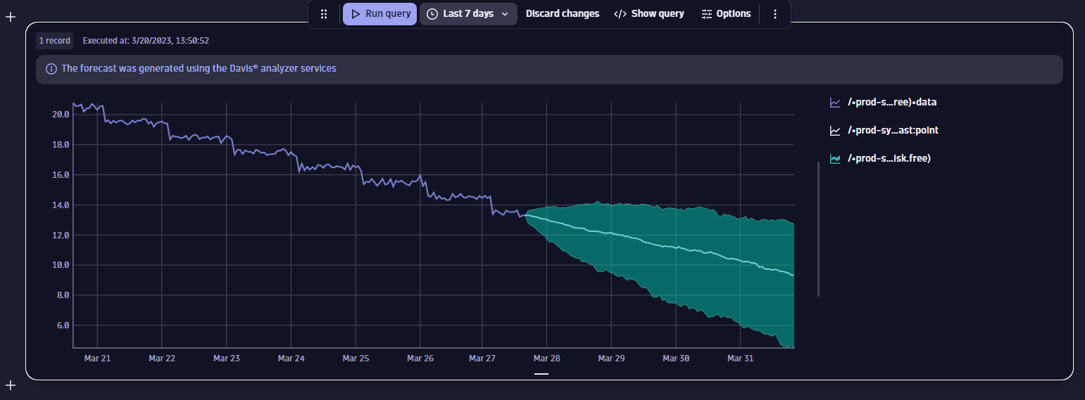
Seasonal data with noise
This example shows the forecast for a 1.5-hour timeframe. Notice that the forecasted interval is not smooth, reflecting the noise in input data.

Seasonal data with noise on an extended timeframe
This example shows the forecast for a 6-hours timeframe. Apart from an extensive forecast timeframe, the data itself has some noise and a downward trend that affect forecast quality—the forecasted interval widens more and more as it goes into the future.
